M721: Index Theory

Examples of Atiyah-Singer Index Theorem

Let’s begin with some notations.

Let $D:C^\infty (E) \rightarrow C^\infty (F)$ be an elliptic differential operator, where $E$ and $F$ are vector bundles over a closed oriented manifold $X^n$ . Suppose $E, F$ and $TX$ have smooth inner product structures. Let $D(X):=D(T^*X)$ and $S(X):=S(T^*X)$ be the disk and sphere bundle of the cotangent bundle, respectively. Let $\pi: D(X)\rightarrow X$ be the projection. Let $[\sigma_D]=[\pi^*E, \pi^*F; \sigma_D]\in K(D(X),S(X))$ be the associated symbol class. Let $\textrm{ch} ([\sigma_D])\in H^{2*}(D(X),S(X);\Bbb{Q})$ be its Chern character. Let $\textrm{td} (X)$ denote the pullback of the Todd class $\pi^*\textrm{td} (T^*X\otimes \Bbb{C})\in H^{2*}(D(X);\Bbb{Q})$ . Let $[D(X)]\in H_{2n}(D(X),S(X))$ be the fundamental class.

Definition. The topological index of $D$ is defined to be $\textrm{t-ind} \ D:=(-1)^n\langle \textrm{ch}[\sigma_D]\textrm{td} (X),[D(X)]\rangle$ .

Atiyah-Singer Index Theorem. $\textrm{ind} \ D=\textrm{t-ind} \ D$ , where $\textrm{ind} \ D:=\textrm{dim}_{\Bbb{C}}(\textrm{ker} D)-\textrm{dim}_{\Bbb{C}}(\textrm{cok} \ D)$ is the analytical index.

Example. [Point Case] Let $X$ be a point. Then $E$ and $F$ are finite dimensional vector spaces. Any non-trivial differential operator $D$ is a linear map between them, and hence of order 0. Thus, $\sigma_D=D$ . Note that $D(X)=X, S(X)$ is empty set. Recall the definition of Chern character, then we have $\textrm{ch} (E)=\textrm{dim} E$ and $\textrm{ch} (F)=\textrm{dim} F$ . Since $S(X)$ is empty set, then $[\sigma _D]=[E]-[F]$ and hence $\textrm{ch} ([\sigma _D])=\textrm{dim} E-\textrm{dim} F$ . Recall the definition of Todd class, we then have $\textrm{td} (X)=1$ . Therefore, by the definition of topological index, we have $\textrm{t-ind} \ D=\textrm{dim} E-\textrm{dim} F$ . By Atiyah-Singer, $\textrm{dim} (\textrm{ker} D)-\textrm{dim} (\textrm{cok} \ D)=\textrm{dim} E-\textrm{dim} F$ .

Example [ $S^1$ Case] Let $X=S^1=\Bbb{R}/2\pi\Bbb{Z}$ , $E=F=S^1\times\Bbb{C}$ , $D=\frac{d}{dx}: C^\infty(S^1,\Bbb{C})\rightarrow C^\infty(S^1,\Bbb{C}).$ Then $D$ is a first order elliptic operator. We now claim that $\textrm{ind} \ D=0$ . We give four different proofs.
Proof 1. We compute $\textrm{ind} \ D$ directly. Note that $\textrm{ker} \frac{d}{dx}=\{constant functions\}$ and that $\textrm{cok} \ \frac{d}{dx}\xrightarrow{\approx}\Bbb{C}$ via $[f]\mapsto\int_{S^1}f$ .
Proof 2. Since $E=F$ , we have $[\sigma_D]=[\pi^*E,\pi^*F;\sigma_D]=[\pi^*E\cup_{\sigma_D}\pi^*F]-[\pi^*F\cup_{\textrm{id}}\pi^*F]=[\pi^*F\cup_{\textrm{id}}\pi^*F]-[\pi^*F\cup_{\textrm{id}}\pi^*F]=0.$
Proof 3. $\textrm{ind} \ \frac{d}{dx}=\textrm{ind} \ i\frac{d}{dx}=0$ , since $i\frac{d}{dx}$ is self-adjoint.
Proof 4. We will show that the topological index vanishes whenever $n$ is odd. See next example.

Example [Odd Dimensional Case, Theorem 13.12 in Lawson-Michaelson]
We will show that the topological index of any elliptic differential operator vanishes whenever $n$ is odd.

We want to show that $\textrm{t-ind} \ D =-\textrm{t-ind} \ D$ , where $D$ is an elliptic differential operator of order $m$ . Consider the diffeomorphic involution $c: TX\rightarrow TX$ given by $c(v)=-v$ . Since
$\textrm{t-ind}\ D=-\textrm{ch} ([\sigma_D])\textrm{td} (X)[D(X)]$

$\ \ \ \ \ \ \ \ \ \ \ \ =-\textrm{ch} ([\sigma_D])\textrm{td} (X)c_*c_*[D(X)]$

$=-c^*(\textrm{ch} ([\sigma_D])\textrm{td} (X)) c_*[D(X)]$

$=-(\textrm{ch} (c^*[\sigma_D]))\textrm{td} (X) (-[D(X)])$ ,
it suffices to show $c^*[\sigma_D]=[\sigma_D]$ . In fact, $c^*[\sigma_D]=[\pi^*E,\pi^* F;(-1)^m\sigma_D]=[\pi^*E,\pi^* F;\sigma_D]=[\sigma_D]$ , since $\sigma_D$ is homotopic to $-\sigma_D$ via $e^{i\pi t}D, t\in [0,1]$ .
Next, we need to introduce the Thom Isomorphism to talk about the de Rham operator.

Let $E$ be an oriented $\Bbb{R}^k$ -vector bundle over $X$ , with inner product on each fiber. We now give the notion of Thom class and Thom space.

Definition. $u(E)\in H^k(D(E)),S(E))$ is a Thom Class of $E$ if it restricts to a generator of $H^k(D^k,S^{k-1})\approx H^k(\pi^{-1}\{x\}\cap D(E),\pi^{-1}\{x\}\cap S(E))$ on each fiber. The quotient $D(E)/S(E)$ is called the Thom space of $E$ , and denoted by $\textrm{Th} (E)$ .

Thom Isomorphism Theorem. The composition $H^*(X)\xrightarrow{\approx}H^*(D(E))\xrightarrow{\smallsmile u}H^{*+k}(D(E),S(E))$ is an isomorphism.

We denote the composition by $\textrm{-}\smallsmile u : H^*(X)\xrightarrow{\approx}H^{*+k}(D(E),S(E))=\widetilde{H}^{*+k}(\textrm{Th}(E))$ and denote its inverse by $\pi_!$ .

Remark. $\pi_!$ has the following two other interpretations.

(1). Integration over the fiber. $\pi_! : \Omega^{i+k}(E)\rightarrow\Omega^i(X)$ , where $E$ is a $\Bbb{R}^k$ bundle over $X$ .
Let $\tau\in\Omega^{i+k}(E)$ be given and choose $x\in X$ and $v_1,...,v_i\in T_xX$ . Associated to these data is a form $\tau^{x,v_1,...,v_i}\in\Omega^k(E_x)$ , defined as follows. Given $e\in E_x$ and a basis $e_1,...,e_k\in T_e E_x$ , choose lifts $\widetilde{v_l}\in T_e E_x$ such that $d\pi (e)\widetilde{v_l}=v_l$ , for each $l\leq i$ , and define

$(\tau^{x,v_1,...,v_i})_e(e_1,...,e_k):=\tau_e(\widetilde{v_1},...,\widetilde{v_i},e_1,...,e_k).$ Now $\pi_! \tau\in\Omega^k(X)$ is defined by

$(\pi_!\tau)_x(v_1,...,v_i):=\int_{E_x}\tau^{x,v_1,...,v_i}.$

Integrating over the fibers will give the second formulation of the topological index, which is the next theorem. The factor $(-1)^{\frac{n(n+1)}{2}}$ compensates for the difference between the orientation on $TX$ induced by the one on $X$ , and the canonical orientation on $TX$ inherited from its almost complex structure.

(2) . Also, we can use the second interpretation of $\pi_!$ to give that formulation.

$\pi_!$ is the composition (Poincare duality) $\ \circ\ \pi_*\ \circ$ (Poincare-Lefschetz duality),

$H^{*+k}(D(E),S(E))\rightarrow H_{n-*}(D(E))\xrightarrow{\pi_*} H_{n-*}(X)\rightarrow H^*(X).$
Then, we compute
$\textrm{t-ind}\ D=(-1)^n \textrm{ch}[\sigma_D]\textrm{td} (X)[D(X)]$
$=(-1)^{\frac{n(n+1)}{2}}\textrm{td} (X) \pi_*(\textrm{ch} ([\sigma_D])\smallfrown [D(X)])$
$= (-1)^{\frac{n(n+1)}{2}}\textrm{td} (X) \pi_!(\textrm{ch} ([\sigma_D])\smallfrown [X])$
$= (-1)^{\frac{n(n+1)}{2}}\pi_!( \textrm{ch} ([\sigma_D]))\textrm{td} (X)\ [X]$ .

Theorem. $\textrm{t-ind} \ D=(-1)^{\frac{n(n+1)}{2}}\pi_!( \textrm{ch} ([\sigma_D]))\textrm{td} (X)\ [X]$ .

We will then give the third formulation of the topological index. To do this we need the notion of Euler class.

Definition. The Euler class of an oriented $\Bbb{R}^k$ -bundle over $X$ , denoted by $latexe(E)$, is the image of the Thom class $u$ under the following isomorphism: $H^k(D(E),S(E))\xrightarrow{i^*}H^k(D(E))\xrightarrow{\approx}H^k(X)$ . We may denote the composition by $i^*$ .

Theorem. [Gysin Sequence] To any bundle $E$ as above there is associated an exact sequence of the form $\cdots\rightarrow H^i(X)\xrightarrow{\smallsmile e(E)} H^{i+k}(X)\xrightarrow{\pi^*} H^{i+k}(S(E))\rightarrow H^{i+1}(X)\xrightarrow{\smallsmile e}\cdots.$

Definition. The Euler characteristic of $X$ is defined to be $\chi (X):=\langle e(TX),[X]\rangle.$

From now on, we assume $n=2m$ .

We want to analyze $\pi_!\textrm{ch}([\sigma_D])$ to give the third formulation of the topological index. For details please see Lawson-Michaelson, P258, Theorem 13.13.

Since – $\smallsmile u$ and $\pi_!$ are inverse to each other, we have $(\pi_!\textrm{ch}([\sigma_D]))\smallsmile u(TX)=\textrm{ch}([\sigma_D])$ . Applying $i^*$ to both sides, we then get $(\pi_!\textrm{ch}([\sigma_D]))\smallsmile e(TX)=i^*\textrm{ch}([\sigma_D])=\textrm{ch} (i^*\sigma_D])=\textrm{ch}(E)-\textrm{ch}(F).$ Thus we can write $\pi_!\textrm{ch}([\sigma_D])=\frac{\textrm{ch}(E)-\textrm{ch}(F)}{e(TX)}$ , if $e(TX)\neq 0$ .

Theorem. $\textrm{t-ind} \ D=(-1)^{\frac{n(n+1)}{2}}\frac{\textrm{ch}(E)-\textrm{ch}(F)}{e(TX)}\textrm{td} (X)\ [X]$ , if $e(TX)$ is not zero.

Now, we are trying to apply this formula to the de Rham operator.

Example. [de Rham operator] Let $\Omega^k_\Bbb{C}=C^\infty(\Lambda^k\ T^*X\otimes \Bbb{C}).$ Then we already know that $(\Omega_\Bbb{C}^\bullet, d)$ is an elliptic complex, that $d: \Omega_\Bbb{C}^{even}\rightarrow\Omega_\Bbb{C}^{odd}$ is an elliptic operator and that $\textrm{ind} \ d=\Sigma(-1)^i\ \textrm{rk}(H^i_{DR}(X))$ . We want to use the above theorem to show that $\textrm{t-ind}\ d=\Sigma (-1)^i \ \textrm{rk}( H^i(X)),$ the Euler charateristic.

For a complex vector bundle $E$ , by the splitting principle, we can write $E$ as $\oplus_i L_i$ . Then $\Sigma_0^n \Lambda^i E=\otimes_1^n\Lambda L_i=\otimes_1^n (\Bbb{C}\oplus L_i)$ . It follows that $\textrm{ch} (\Sigma_0^n \Lambda^i E)=\prod_1^n (1+e^{x_i}).$ Similarly, we have $\textrm{ch} (\Sigma_0^n (-1)^i\Lambda^i E)=\prod_1^n (1-e^{x_i}).$

Back to our example, applying the real splitting principle to $T^*X$ , we compute

$\textrm{ch} (\Sigma (-1)^i \Lambda^i T^*X\otimes\Bbb{C})=\prod_1^n (1-e^{x_i})=\prod_1^n (1-e^{-x_i}),$

since $x_i=-x_{i+m}$ for $1\leq i\leq m$ . Note that $\textrm{td} (X)=\prod_1^n \frac{x_i}{1-e^{-x_i}}$ , and that $e=\prod_1^m x_i$ , then by the theorem above, we obtain

$\textrm{t-ind} \ d=(-1)^{\frac{n(n+1)}{2}}\frac{\prod_1^n (1-e^{-x_i})}{\prod_1^m x_i}\prod_1^n \frac{x_i}{1-e^{-x_i}} [X]=(-1)=\prod_1^m x_i [X]=\chi (X).$

Written by topoclyb

January 13, 2013 at 7:37 pm

Posted in Uncategorized

The index theorem for the signature and Dirac operators

leave a comment »

This post will be converted into WordPress later. In the meantime, view it in PDF form here: DiracIndexTheory

Written by Henry T. Horton

December 15, 2012 at 3:43 pm

Posted in Uncategorized

The Dirac operator

with one comment

We begin by endowing a vector bundle with a Clifford module structure. It is with additional structure that we may define a Dirac operator.

Let $(X^n, g)$ be an $n$ -dimensional Riemannian manifold with covariant derivative $\nabla^X$ (on $TX$ ) , and let $\mathbb{R}^N\to S\to X$ be a vector bundle.

Clifford Module Bundles and a Dirac “Type” Operator

Definition (Clifford module)

A Clifford module $T$ for a real inner product space $(V,\beta)$ is a left module over $Cl(V,\beta)$ . Equivalently, there is a -algebra homomorphism $c: Cl(V,\beta) \to \text{Hom(T,T)}$ given by $c(v) = (t\mapsto v\cdot t)$ . Since $v^2:=v\cdot v = -||v||^2$ for any $v\in Cl(V,\beta)$ (see the Glossary below), one has that $c$ satisfies $c(v)^2 = - ||v||^2\text{Id}$ .

Definition (Bundle of Clifford Modules)

A bundle $S$ (as above) is a bundle of Clifford modules if there is a map of bundles of $\mathbb{R}$ -algebras $C:Cl(TX)\to \text{Hom}(S,S)$ such that $c(v)^2s = -||v||^2 s$ for any section $s\in C^{\infty}(S)$ . In other words, for each $x\in X$ , $\text{Hom}(S_x, S_x)$ is a Clifford module for $(T_x X, g_x)$ .

Definition (Dirac type operator)

Let $S$ be a Clifford module bundle equipped with a covariant derivative $\nabla^S$ . Let $D:C^\infty(S)\to C^\infty(S)$ be the map defined by the composition

$C^\infty(S)=\Omega^0(S) \xrightarrow{\nabla^S} \Omega^1(S) = C^\infty(\text{Hom}(TX,S)) \xrightarrow{H} C^\infty(TX\otimes S)\xrightarrow{c} \Omega^0(S)$

where $H$ is the inverse of the bundle isomorphism $C^\infty(TX\otimes S) \to C^\infty(\text{Hom}(TX,S)), v\otimes s \mapsto g(v,.)\otimes s$ , and where $c(v\otimes s) = v\cdot s$ is Clifford multiplication. We call such a map (which depends on the Clifford module bundle $S$ , $\nabla^S$ and $g$ ) a Dirac type operator.

If we a fix an orthonormal frame $\{e_1,\ldots, e_n\}$ for $TX$ over some neighborhood $U\subset X$ and, using the metric $g$ , let $\{e^i\}$ be the corresponding frame for $T^\ast X|_U$ , we may write this composition locally as

$s\overset{\nabla^S}{\mapsto} \sum_{i=1}^n e^i\otimes \nabla^S_{e_i} s \overset{H}{\mapsto} \sum_{i=1}^n e_i\otimes \nabla^S_{e_i} s \overset{c}{\mapsto} \sum_{i=1}^n e_i\cdot \nabla^S_{e_i} s$

That is, a Dirac type operator is locally of the form

$Ds = \sum_{i=1}^n e_i\cdot \nabla^S_{e_i} s$ .

Proposition

A Dirac type operator is a first order differential operator.

Proof

Let $s\in C^\infty(S)$ and $f\in C^{\infty}(X)$ . Using the local description above, we compute:

$[D, f]s = D(fs) - f(Ds)$

$= \sum_{i=1}^n \bigl[ e_i\cdot \nabla^S_{e_i} (fs) - f e_i\cdot \nabla^S_{e_i} s\bigr]$

$= \sum_{i=1}^n \bigl[ e_i\cdot (e_i(f)s + f \nabla^S_{e_i} s) - f e_i\cdot \nabla^S_{e_i} s\bigr]$

$= \sum_{i=1}^n \bigl[ e_i\cdot e_i(f)s + e_i\cdot f \nabla^S_{e_i} s - f e_i\cdot \nabla^S_{e_i} s \bigr]$

$= \sum_{i=1}^n \bigl[ e_i\cdot e_i(f)s + f e_i\cdot \nabla^S_{e_i} s - f e_i\cdot \nabla^S_{e_i} s \bigr]$

$= \sum_{i=1}^n e_i\cdot e_i(f)s$ .

In particular, $[D,f](gs) = g[D,f](s)$ for $g\in C^{\infty}(X)$ , so $[D,f]$ is $C^\infty(X)$ -linear and hence in $DO_0(S,S)$ . Thus $D\in DO_1(S,S)$ , and as $D$ itself is not $C^\infty(X)$ -linear, $D$ is of order 1. $\square$

Remark

The above proof extends (by incorporating induction) to show that the composition of a $k$ – and an $m-$ order differential operator is a differential operator of order $\leq k+m$ . Here, $\nabla^S$ and $c$ are differential operators of order 1 and 0, respectively.

We next show that $D$ is elliptic.

Lemma (Symbol of a Dirac type operator)

Let $D$ be a Dirac type operator and let $\xi^\ast\in T^\ast X$ . Then the symbol $\sigma_D(\xi^\ast)$ of $D$ at $\xi^\ast$ is given by

$\sigma_D(\xi^\ast)(s) = \frac{1}{i} \xi\cdot s$ ,

where $\xi\in TX$ is the dual to $\xi^\ast$ determined by the metric, i.e., such that $\xi^\ast = g(\xi, \cdot)$ .

Proof

Fix $x\in X$ , and let $U$ be an open neighborhood of $x$ in $X$ . Using $g$ choose an orthonormal frame $\{e_i\}$ of $TX|_U$ with dual frame $\{e^i\}$ for $T^\ast X|_U$ . Being a bundle homomorphism $\pi^\ast(S)\to \pi^\ast(S)$ (over $\mathbb{R}$ ), $\sigma_D$ is $\mathbb{R}$ -linear in the $T^\ast X$ -ordinate. Thus it suffices to verify the proposition for $e^j$ ; that is, we wish to show that $\sigma_D(e^j)(s) = \frac{1}{i} e_j\cdot s$ for $s\in C^{\infty}(S|_U)$ .

Choose a local chart $\varphi: U\to \mathbb{R}^n$ such that $\varphi(x)=0$ ; let $x_i=\text{pr}_i\circ \varphi: U\to \mathbb{R}$ . Note that $\{e_i(x)\}$ is an orthonormal basis for $T_xX$ . Let $\frac{\partial}{\partial x_i} = d\varphi_x(e_i(x))$ ; then ${dx_j}_x(e_i(x)) = {d\text{pr}_j}|_0\circ d\varphi_x(e_i(x)) = {d\text{pr}_j}|_0\bigl(\frac{\partial}{\partial x_i}\bigr) = \delta_{ji}$ , so ${dx_j}_x = e^j(x)$ .

Thus (see the Glossary below), as $D$ is order $1$ , we have

$\sigma_D(e^j)(s(x)) = \frac{1}{i} D(x_j s)(x)$

$= \frac{1}{i} (\sum_{i=1}^n e_i\cdot \nabla_{e_i}(x_j s))(x)$

$= \frac{1}{i} \sum_{i=1}^n e_i(x) \cdot \bigl[ {dx_j}_x(e_i(x)) s(x) + \underbrace{x_j(x)}_{=0}\nabla_{e_i}s(x)\bigr]$

$= \frac{1}{i} \sum_{i=1}^n e_i(x) \cdot \bigl[ \delta_{ji} s(x) + 0]$

$= \frac{1}{i} e_j(x)\cdot s(x)$ ,

as required. $\square$

Corollary

A Dirac type operator is elliptic.

Proof

If $\xi^\ast\in TX^\ast-X$ then $\sigma_D(\xi^\ast)$ has inverse $\sigma_D^{-1}(\xi^\ast)(s) = i \frac{1}{\xi^\ast} \cdot s$ . $\square$

Remark

Noting that $\sigma_{D^2}(\xi) = \sigma_D(\xi)\sigma_D(\xi)$ (the product of linear maps), we observe that $\sigma_{D^2}(\xi)s = -\xi\cdot \xi \cdot s = ||\xi||^2 s$ . Taking $S=Cl(TX)$ , this — apparently — implies that a Dirac type operator is, at the symbol level, the square root of the Laplacian.

$\mathbb{Z}_2$ -grading and “a” Dirac Operator

A Dirac type operator is formally self-adjoint (so that its index is $0$ ) if we impose the following further restrictions on the Clifford-module bundle.

Definition (Clifford-Compatible)

Let $S\to X$ be a bundle of Clifford modules. We say that $S$ is Clifford compatible if it is equipped with a metric $\langle, \rangle$ and a covariant derivative $\nabla^S$ such that

(1) $\nabla^S$ is Riemannian, i.e., for all sections $s, t\in C^\infty(S)$ :

$d\langle s, t\rangle = \langle \nabla^S s, t\rangle + \langle s, \nabla^S t \rangle$ , and

(2) for all vector fields $V, W\in C^{\infty}(TX)\subset C^{\infty}(Cl(TX))$ and for any section $s\in C^\infty(S)$ :

$\nabla^S_V(W\cdot s) = \nabla^X_V W \cdot s + W\cdot \nabla^S_V s$ .

Definition (A Dirac operator)

A differential operator $D: C^\infty(S)\to C^\infty(S)$ is a Dirac operator if

(1) $D$ is a Dirac type operator, and

(2) $S$ is Clifford compatible.

Lemma

If $X$ is oriented and $D$ is a Dirac operator, then $D$ is formally self-adjoint. That is,
$\langle\langle Ds, t\rangle\rangle = \langle\langle s, Dt\rangle\rangle$ ,
where $\langle\langle s,t\rangle\rangle = \int_{X} \langle s, t \rangle$ (and the integration is with respect to the volume form on $X$ ).

Proof

Omitted 😦 $\square$

Consequently we have $\text{index}(D)=0$ (see Ning’s blog). To make use of the index, then, we introduce a $Z_2$ -grading on Clifford module bundles.

Definition

Recall that a Clifford algebra is $\mathbb{Z}$ -filtered — $Cl_n=\cup_{i} {Cl_n^i}$ with $Cl_n^i\cdot Cl_n^j\subset Cl_n^{i+j}$ — and $\mathbb{Z}_2$ -graded — $Cl_n={Cl_n}^{+}\oplus {Cl_n}^-$ (even and odd products).

A Clifford module bundle $S$ is $\mathbf{Z}_2$ -graded if it decomposes into a direct sum $S=S^+\oplus S^-$ of vector bundles such that for each $x\in X$ and $v\in T_xX$ , one has $v\cdot S_x^{\pm} \subset S_x^{\mp}$ .

Such a $\mathbb{Z}_2$ -graded bundle is compatible if this decomposition is both orthogonal with respect to $\, \langle, \rangle$ and parallel with respect to the covariant derivative $\nabla^S$ , ie. $\nabla^S S^{\pm} \subset S^{\pm}$ .

Example

If $X$ is oriented, the Clifford bundle $Cl(TX) = Cl^+(TX) \oplus Cl^-(TX)$ is a $\mathbb{Z}_2$ -graded compatible Clifford bundle. Some words which may be connected to verify this: Levi Civita connection, induced connection on $F(TX)$ , lift to principal spin bundle, induced covariant derivative on associated vector bundle, compatibility with the metric.

Examples of Dirac Operators

We now look at four examples of Dirac operators. The first two are familiar; here we reinterpret them in terms of Clifford modules.

Example 1: The De Rham Operator

Recall that the filtered algebra $Cl(V^n,q) = \cup Cl^i(V,q)$ has associated graded algebra $Gr(Cl(V,q))\cong \Lambda^\ast V$ . (See the Glossary below.)

Lemma

Let $f:\Lambda^\ast(\mathbb{R})\to Cl_n(\mathbb{R})$ be the map defined by

$v_1\wedge \ldots \wedge v_r\mapsto \frac{1}{r!} \sum_{\sigma\in \Sigma_r} \text{sign}(\sigma) v_{\sigma(1)}\cdot v_{\sigma(2)}\cdots v_{\sigma(r)}$ .

Then $f$ is

(1) an isomorphism of vector spaces

(2) filtration preserving, i.e., $f(\oplus_{i\leq r} \Lambda^i(\mathbb{R}))\subset {Cl_n}^r(\mathbb{R})$ , and

(3) $O(n)$ -equivariant, i.e., $f(A\omega) = A f(\omega)$ for $\omega\in \Lambda^\ast(\mathbb{R})$ and $A\in O(n)$ .

Proof

(1) and (2). Let $e_1, \ldots, e_n$ is an orthonormal basis for $\mathbb{R}^n$ . Since (by an equivalent definition of the exterior algebra) $v_1\wedge \ldots \wedge v_r = \frac{1}{r!} \sum_{\sigma\in \Sigma_r} \text{sign}(\sigma) v_{\sigma(1)}\otimes v_{\sigma(2)}\otimes\ldots \otimes v_{\sigma(r)}$ , we see that $f$ is induced by the map $T(\mathbb{R}^n) \to Cl_n(\mathbb{R})$ taking $e_{i_1}\otimes \cdots\otimes e_{i_r}$ to $e_{i_1}\ldots e_{e_r}$ and descending to $\Lambda^\ast(V)$ ; that is, $f(e_{i_1}\wedge\ldots \wedge e_{i_r}) = e_{i_1}\cdots e_{i_r}$ . It follows that $f$ is an isomorphism and preserves the grading.

(3) Using that $Ae_1\wedge \ldots Ae_n = (\text{det} A) (e_1\wedge \ldots e_n)$ , I feel like we need to be working with $SO(n)$ here. Please comment! $\square$

Corollary

The exterior algebra bundle over a(n oriented?) manifold $\Lambda^\ast(T^\ast X)$ and the clifford bundles $Cl(TX)$ are isomorphic as vector bundles.

Proof

Let $F(TX)$ denote the principal $O(n)$ -bundle associated to $TX$ . By parts (1) and (3) of the lemma, the map $f$ above induces a vector bundle isomorphism $\Lambda^\ast(TX) = F(TX)\times_{O(n)} \Lambda^\ast(\mathbb{R}^n) \to F(TX)\times _{O(n)} Cl_n(\mathbb{R}) = Cl(TX)$ . $\square$

Theorem 2.5.12 (Lawson, Michelsohn)

Under this bundle isomorphism $\Lambda^\ast(T^\ast X) \cong Cl(TX)$ , the de Rham operator $d+d^\ast$ corresponds to the Dirac operator $D$ .

Corollary

Since we have already established (see Hailiang’s(?) blog post) that the Euler characteristic $\chi(X)$ of $X$ is equal to $\text{Index}(d+d^\ast|_{\Omega^{\text{even}}}:\Omega^{\text{even}}\to \Omega^{\text{odd}})$ , the theorem (along with the grading-preserving property of $f$ ) implies we may also compute it as $\text{Index}(D|_{C^\infty(Cl^+(TX))}: C^\infty(Cl^+(TX))\to C^\infty(Cl^-(TX)))$ .

Example 2: The Signature Operator

We now look to reinterpret the signature operator in terms of Clifford bundles.

Recall (see Hailiang’s blog) in the case that $n=2p$ and $p$ is even, the Hodge star operator $\ast: \Omega^p\to \Omega^{n-p}$ is an involution so we can decompose $\Omega^p = \Omega^p_+\oplus \Omega^p_-$ into the $+1$ and $-1$ eigenspaces of $\ast$ . We defined the signature operator $D = d+d^\ast$ . Since $D\ast = -\ast D$ , we saw that $D$ took $\Omega^p_{\pm}$ to $\Omega^p_{\mp}$ and letting $D_+=D|_{\Omega^p_+}$ , we found that $\text{Index}(D_+) = \text{Sign}(X)$ . The signature $\text{sign}(X)$ of $X$ was defined to be the signature of the quadratic form on $\mathcal{H}^p$ given by $(\alpha,\beta)\mapsto \int_X \alpha\wedge \beta$ .

In the case that $p$ is odd, we had to modify the construction. We complexified, taking $\Omega_\mathbb{C}^p = C^\infty(\Lambda^p(T^\ast X\otimes \mathbb{C}))$ , and defined $\tau = i\ast$ . Then the above paragraph went through with $\tau$ replacing $\ast$ and $\Omega_\mathbb{C}$ replacing $\Omega$ .

Let $\{e_1, \ldots, e_n\}$ be an oriented orthonormal basis for $\mathbb{R}^n$ . Let $\omega = e_1\cdots e_n$ in $Cl_n$ . Then by the lemma above and the corresponding properties of the volume form $e_1\wedge\ldots \wedge e_n$ in $\Lambda^\ast(\mathbb{R}^n)$ , we obtain that $\omega$ is a basis-independent section of $Cl_n(\mathbb{R})$ .

Lemma

(1) We have $\omega^2 = \begin{cases} 1 \qquad n\equiv 0, \, 3 \mod 4\\ -1 \qquad n\equiv 1, \, 2 \mod 4 \end{cases}$

(2) If $n$ is even and $v\in \mathbb{R}^n$ , then $\omega \cdot v = -v \cdot \omega$ .

Proof

(1) We compute $(e_1\cdots e_n)(e_1\cdots e_n) = (-1)^n(-1)^{n-1}\cdots (-1)^2 (-1)^1 = (-1)^{n(n+1)/2}$ . Writing $n=4k+l$ for $0\leq l\leq 3$ , one finds that $n(n+1)/2$ is even if and only if $l=0$ or $3$ .

(2) It suffices to verify for $v=e_i$ . We have $(e_1\cdots e_n)\cdot e_i = (-1)^{n-i} e_1\cdots \hat{e}_i\cdots e_n$ and $e_i \cdot (e_1\cdots e_n) = (-1)^i e_1\cdots \hat{e}_i\cdots e_n$ . (Here, a hat $\hat{}$ indicates that the element be omitted from the product.) Since $n$ is even, $(-1)^{n-i}=(-1)^i$ . $\square$

Now, $\omega$ acts on any Clifford module via $v\mapsto w\cdot v$ , and by part (1) of the lemma this defines an involution in the case $n\equiv 0, 3\mod 4$ ; in the case $n\equiv 1, 2\mod 4$ , $i\omega$ defines an involution. Compare with the Hodge star operator recalled above. So define

$\Gamma = \begin{cases} \omega \qquad n\equiv 0, \, 3 \mod 4,\\ i\omega \qquad n\equiv 1, \, 2 \mod 4; \end{cases}$

then $\Gamma^2=\text{Id}$ . Thus if $X$ is an oriented manifold and $S$ is a Clifford module bundle of $X$ , putting $S^{\pm} = \{v\in S: \Gamma v = \pm v\}$ , we have

if $n\equiv 0, 3 \mod 4$ : $S = S^+\oplus S^-$ , or

if $n\equiv 1,2 \mod 4$ : $S_\mathbb{C} = S_\mathbb{C}^+\oplus S_\mathbb{C}^-$

Corollary

If $n$ is even then $S$ is $\mathbb{Z}_2$ -graded, i.e., for $x\in X$ and $v\in T_xX$ , one has $v\cdot S_x^{\pm} \subset S_x^{\mp}$ .

Proof

By part (2) of the lemma, for $v\in T_xX$ we have $\Gamma v = -\Gamma v$ .
Thus if $e\in S_x^{\pm}$ (i.e. $\Gamma e = \pm e$ ) then $v\cdot e = v\cdot (\pm \Gamma(e)) = \mp \Gamma(v\cdot e)$ , so $v\cdot e\in S^{\mp}$ . $\square$

Proposition

If $n$ is even and $S$ is $\mathbb{Z}_2$ -graded compatible, then the associated Dirac operator splits as
$D = \left( \begin{array}{cc}0 & D^-\\ D^+ & 0\end{array}\right): C^\infty S^+\oplus C^\infty S^-\to C^\infty S^+\oplus C^\infty S^-$ .
In particular, if $S=Cl(TX)$ , by Theorem 2.5.12 we have $\text{Index}(D^+) = \text{Sign}(X)$ .

Proof

Since $S$ is $\mathbb{Z}_2$ -graded and is compatible (so in particular, the covariant derivative preserves $S^{\pm})$ , the Dirac operator
$Ds = \sum e_i\cdot \nabla_{e_i}^S s$
takes $C^\infty(S^{\pm})$ to $C^\infty(S^{\mp})$ . $\square$

Example 3: twisted Dirac Operators

Preliminary: If $S$ and $E$ are vector bundles over $X$ with covariant derivatives $\nabla^S$ and $\nabla^E$ , respectively, then the tensor product bundle $S\otimes E\to X$ has covariant derivative
$\nabla^S\otimes \nabla^E := \text{Id}_S\otimes \nabla^E + \nabla^S\otimes \text{Id}_E$ .

Fact: If $S$ is a compatible $\mathbb{Z}_2$ -graded Clifford module bundle and $(E, g, \nabla^E)$ is a Riemannian bundle (see Property (1) of a compatible Clifford Bundle above for the definition), then $S\otimes E$ is a compatible $\mathbb{Z}_2$ -graded Clifford module bundle (with Clifford multiplication $v\cdot(s\otimes e) = (v\cdot s)\otimes e$ for $v\in Cl_n$ , $s\in S$ , $e\in E$ ). In the case that $S=Cl(TX_{\mathbb{C}})$ , we call the Dirac operator on $S\otimes E$ a twisted Dirac operator.

Fact: (Apparently from topological K-theory) If the Index theorem holds for any twisted Signature operator then it holds for all elliptic differential operators.

Example 4: Spin Manifolds and The Atiyah-Singer Dirac Operator

Recall (see Prasit’s blog) that there is an isomorphism $\varphi: Cl_{2l}(\mathbb{C}) \xrightarrow{\cong} M_{2^l}(\mathbb{C})$ . So since
$\mathbb{C}^n$ is an $M_n(\mathbb{C})$ module, one has that $\mathbb{C}^{2^l}$ is an $Cl_{2l}(\mathbb{C})$ -module via $a\cdot v = \varphi(a)v$ , for $a\in Cl_{2l}(\mathbb{C})$ and $v\in \mathbb{C}^{2^l}$ . To avoid confusion, let us call $\mathbb{C}^{2^l}$ with this module structure $C$ .

Now, any $M_{2^l}(\mathbb{C})$ -module is isomorphic to $\oplus^{2^l} \mathbb{C}^{2^l}$ , so it follows that any $Cl_{2l}(\mathbb{C})$ -module is isomorphic to $\oplus^{2^l} C$ .

Let $S$ be a Clifford module bundle. From the above paragraph we see that each fiber (a $Cl_{2l}(\mathbb{C})$ -module) is isomorphic (via $\varphi_x$ , say) to $\oplus^{2^l} C_x$ , where $C_x$ is a copy of $C$ . We may then
ask if this splitting extends over the whole bundle; that is, is there a Clifford module bundle $S\to X$ and a bundle isomorphism $\varphi:S\to \oplus^{2^l} C$ which restricts fiberwise to an isomorphism $S_x\cong \oplus^{2^l} C$ .

In turns out the answer is a resounding “Yes” if $X$ is a spin manifold.

Definition (Spin Structure)

Let $E\to X$ is an $N$ -dimensional vector bundle. A spin structure on $E$ is a principal $\text{Spin}(N)$ -bundle $P\to X$ together with a bundle isomorphism $P\times_{\text{Spin}(N)} \mathbb{R}^N\to E$ . (Then $E$ is the associated vector bundle for $P$ ). Using classifying space theory, we may reinterpret this
to say that a spin structure on $E$ is a lift of the classifying map $\varphi_E: X\to BGL_N(\mathbb{R})$ to $B\text{Spin}(N)$ .

We may break up the existence of a spin structure into pieces as follows.

After choosing a metric on $E$ , we may first reduce the structure group of $E$ to $O(n)$ . (The only obstruction to doing so is the paracompactness of $X$ .) So we’re left to lift a map $\varphi_E: X\to BO(n)$ to $B\text{Spin}(N)$ .

Since $B\text{Spin}(N)$ is the universal cover of $BSO(N)$ , we may first try to lift $\varphi_E$ to $BSO(n)$ .

The short exact sequence of groups $1\to SO(N)\to O(N)\xrightarrow{\text{det}} \mathbb{Z}_2\to 1$ induces a fibration of classifying spaces
$X\xrightarrow{\varphi_E} BO(N)\to B\mathbb{Z}_2=K(\mathbb{Z}_2,1)$ .

It turns out that the map $X\to BO(N)$ lifts to $BSO(N)$ if and only if the composite $X\xrightarrow{\varphi_E} BO(N)\to B\mathbb{Z}_2=K(\mathbb{Z}_2,1)$ is nullhomotopic. Since $[X, K(\mathbb{Z}_2,1)]\cong H^1(X;\mathbb{Z}_2)$ , there is an element $\omega_1(E)\in H^1(X;\mathbb{Z}_2)$ that vanishes if and only if $\varphi_E$ lifts. We call $\omega_1(E)$ the first Stiefel Whitney class of $E$ .

Similarly, the map $X\to BSO(N)$ lifts to $B\text{Spin}(N)$ if and only if the composition $X\to BSO(N)\to B K(\mathbb{Z}_2,1)=K(\mathbb{Z}_2,2)$ is nullhomotopic; we call the corresponding element in $H^2(X;\mathbb{Z}_2)\cong [X, K(\mathbb{Z}_2,2)]$ (that vanishes iff $X\to BSO(N)$ lifts) the second Stiefel Whitney class $\omega_2(E)$ of $E$ .

Definition (Spin manifold)

We will call an oriented manifold $X$ (so $\omega_1(TX)=0$ ) a spin manifold if its tangent bundle $TX$ admits a spin structure (i.e., $\omega_2(TX)=0$ ). It can be shown that this is equivalent to the existence of a trivialization of $TX$ over the $2$ -skeleton of $X$ . (Compare with the fact that $X$ is orientable if and only if $TX$ is trivializable over the $1$ -skeleton.)

Definition (The Atiyah-Singer Dirac Operator)

Suppose $X^n$ has a spin structure with principal $\text{Spin}(n)$ -bundle $P$ (associated to $TX$ ). Since $Cl_n(\mathbb{C})$ acts on $C$ on the left and $\text{Spin}(n)={Cl_{n}}^+(\mathbb{C})\cap \langle S^{n-1}\rangle$ (where $\langle S^{n-1}\rangle$ has general element $x_1\cdot x_2\cdots x_k$ with $x_i\in \mathbb{C}^n$ , $x_i^2=1$ ) is a subgroup of the group of units $Cl_n^\times$ , we may define
the $C$ -bundle associated to $P$ by $\mathbf{C} = P\times_{\text{Spin}(n)} C\to X$ . Since $C$ is a $Cl_n(\mathbb{C})$ module, $\mathbf{C}$ is a Clifford module bundle.

Some words: By lifting the Levi-Civita connection on $P_{SO(n)}$ one obtains a connection on $P_{\text{Spin}(n)}$ , and hence (see who’s blog?) a covariant derivative $\nabla^\mathbf{C}$ on $\mathbf{C}$ which makes it Clifford compatible
as a $\mathbb{Z}_2$ graded Clifford module bundle.

We may then define the Atiyah-Singer Dirac Operator by

$Ds = \sum e_i\cdot \nabla_{e_i}^\mathbf{C} s$ .

Some more words:

If $Ds=0$ then $s$ is called a harmonic spinor.

If $X$ has positive scalar curvature, then $D$ is injective. So if we have ways to compute the index (using the ASHI theorem, for example), we may be able to deduce that $X$ does not admit a metric of positive scalar curvature.

Glossary

(to include links to other blog posts)

Differential Operator (global definition)

If $E$ and $F$ are vector bundles over $X$ (of the same dimension), we define the family of differential operators of order $\leq m$ from $E$ to $F$ by

$DO_m(E,F) = \{D\in \text{Hom}_{\mathbb{R}}(C^\infty E, C^\infty F):\, [D,f]\in DO_{m-1}(E,F) \, \forall f\in C^{\infty}(X)\}$

with $DO_{-1}(E,F)=\{0\}$ . In particular, $DO_{0}(E,F) = \{C^{\infty}(X)\text{-linear bundle maps } C^\infty(E)\to C^\infty(F)\}$ .

Symbol of a differential operator

(cf. Juanita’s blog) We recall the definition of the symbol $\sigma_D$ of an order- $m$ differential operator $D:C^\infty(E)\to C^\infty(F)$ . Denote $T^\ast X\xrightarrow{\pi} X$ , $E\xrightarrow{p} X$ , so $\pi^\ast(E)=\{(\xi^\ast,e)\in T^\ast X\times E:\, \pi(\xi^\ast)=x=p(e)\}$ . Let $\xi^\ast\in T^\ast X$ . Let $x\in X$ . The symbol $\sigma_D(\xi^\ast)$ of $D$ at $x$ is the homomorphism $E_x\to F_x$ defined by

$\sigma_D(\xi^\ast)(s(x)) = \frac{1}{i} \frac{1}{m!} D(f^m s)(x)$

where $s\in C^\infty(E)$ , and $f\in C^\infty(X)$ is such that $df_x = \xi^\ast(x)$ .

Covariant Derivative

A covariant derivative $\nabla$ on a vector bundle $E\to X$ is a map $\nabla: C^{\infty}(TX)\times C^{\infty}(E)\to C^{\infty}(E)$ , $(v,s)\mapsto \nabla^S_v s$ where $\nabla_v^S$ is an $\mathbb{R}$ -linear map $C^\infty(E)\to C^{\infty}(E)$ satisfying the Leibnitz rule $\nabla^S_v (fs) = v(f)s + f\nabla^S_v(s)$ for $s\in C^\infty(E)$ and $f\in C^\infty(X)$ .

Graded Algebras

(cf Prasit’s blog) A $k$ -algebra $A$ is $\mathbb{Z}$ -graded if $A=\bigoplus_i A_i$ such that $A_i A_j\subset A_{i+j}$ . A $k$ -algebra is filtered over $\mathbb{Z}$
if $A=\cup A^i$ such that $A^i\subset A^{i+1}$ and $A^i A^j \subset A^{i+j}$ . A graded algebra $A=\bigoplus_i A_i$ defines a filtered algebra by taking $A^i=A_0\oplus\ldots A_i$ , and conversely a filtered algebra $A=\cup_i A^i$ defines a graded algebra by taking $A_i=A^i/A^{i-1}$ (with $A^{-1}=0$ ).

Tensor Algebra and the Clifford Algebra

If $V$ is a vector space, the tensor algebra $TV = \mathbb{R}\oplus V\oplus V\otimes V\oplus\ldots \oplus V\oplus\ldots \oplus V$ has multiplication defined by concatenation, i.e., $(x_1\otimes \ldots \otimes x_j)(y_1\otimes \ldots \otimes y_j) = x_1\otimes \ldots \otimes x_j \otimes y_1\otimes \ldots \otimes y_j$ . Thus $TV$ is a graded algebra with $(TV)_i = \underbrace{V\otimes \ldots \otimes V}_{\text{\emph{i} times}}$ , and filtered with $(TV)^i=\mathbb{R}\oplus \cdots \oplus V\otimes\cdots \otimes V$ .

Recall that $Cl(V,q)=\cup_i Cl^i(V,q)$ with $Cl^i(V,q)=(TV)^i/{\langle v\otimes v = -q(v)\rangle}$ . (Here, $q$ is a quadratic form; sometimes it is convenient to refer instead to the associated symmetric bilinear form $\beta$ .) For any $v\in V$ , $q(v)\in \mathbb{R}=Cl^0(V,q)$ so $q(v)$ maps to $0$ under the quotient $Gr_i(Cl(V,q))= Cl^i(V,q)/Cl^{i-1}(V,q)$ . This sets up a natural identification between $Gr_i(Cl(V,q))$ and $(\Lambda^\ast V)_i = \frac{(TV)_i}{\langle v\otimes v=0\rangle}$ . Whence the associated graded algebra for $Cl(V,q)$ is isomorphic to $\Lambda^\ast V$ . In particular, they are isomorphic as vector spaces, with dimension $\sum_{k=0}^n \begin{pmatrix}n\\k\end{pmatrix}=2^n$ .

Clifford bundle

The Clifford bundle $Cl(TX)\xrightarrow{\pi} X$ has fibers $Cl(T_xX, g_x) \cong Cl_n(\mathbb{R})$ ( $x\in X$ ), where $g$ is a Riemannian metric on $X$ . (The latter isomorphism is given by identifying an orthonormal (with respect to $g_x$ ) basis for $T_xX$ with the standard generators $\{e_i\}$ .) Just as $TX$ is the $\mathbb{R}^n$ -bundle associated to the orthogonal frame bundle (of the tangent bundle) $F(TX)$ over $X$ , $Cl(TX)$ is the associated $Cl_n(\mathbb{R})$ -bundle to $F(TX)$ .

Written by aclightf

November 21, 2012 at 7:45 pm

Posted in Uncategorized

Clifford algebras and Spin groups

leave a comment »

As a provisional definition, a clifford algebra over a field ${k}$ can be defined as

$\displaystyle Cl_{n}(k) = k[x_{1}, \ldots, x_{n}] /R$

where,

$\displaystyle R = < x_{i}^{2} = -1, x_{i} x_{j} = - x_{j}x_{i} \forall i \neq j >$

It is easy to see that the clifford algebra has dimension ${2^{n}}$ . It can also be thought of as

$\displaystyle Cl_{n}(k) = TV / R$

where ${V = k^{n}}$ as vector space, ${TV}$ is the tensor algebra, ${R}$ is same as above, except that ${x_{i}}$ ‘s are standard basis for ${V}$ . This observation leads to a more general definition of clifford algebra, where ${V}$ is a vector space equipped with a symmetric bilinear form

Definition 1 Let ${V}$ be a vector space with symmetric biliear form ${\beta}$ and quadratic form ${q = \beta(x,x)}$ . Then the clifford algebra over ${V}$ can be defined as $\displaystyle Cl(V, q) = TV / < x \otimes x + q(x)>$

Remark 1 These are some of the properties that ${CL(V, q)}$ enjoys

There is a natural inclusion of ${i: V \hookrightarrow Cl(V,q)}$ .

If ${q= 0}$ , then ${Cl(V, q) = \bigwedge(V)}$ the exterior algebra

Let ${.}$ denote the clifford multiplication (induced by the tensor product of ${TV}$ ), then $\displaystyle x . y + y . x = -2 \beta(x,y)$

Universal Property : Let ${f: V \longrightarrow A}$ , where ${A}$ is a ${k}$ -algebra, such that ${f(x)^{2} = -q(x)}$ , then there exists an unique ${k}$ -algebra homomorphism ${F : Cl(V,q) \longrightarrow A}$ such that ${f = F \circ i}$ .

A map ${\phi: ( V,q) \longrightarrow (V',q')}$ , such that ${q'(\phi (x)) = q(x)}$ , extends to a ${k}$ -algebra homomorphism $\displaystyle \Phi: Cl(V,q) \longrightarrow Cl(V', q')$ Thus the orthogonal group ${\mathbb{O}(n)}$ has an action on ${Cl_{n}(\mathbb{R})}$

Proposition 2 ${Cl(v,q)}$ is a filtered algebra whose associated graded is ${\bigwedge(V)}$

Before proving the theorem, recall the following definition

Definition 3 If ${A}$ is a ${k}$ -vector space then a filtration ${(A,\mathfrak{F} )}$ of ${A}$ is sequence of subspaces $\displaystyle F_{0}A \subset F_{1}A \subset \dots \subset A = \bigcup_{r}F_{r} A$ so that $F_iAF_jA \subset F_{i+j}A$ .

The associated graded ring of ${(A, \mathfrak{F})}$ is defined as $\displaystyle Gr(A, \mathfrak{F}) = \bigoplus_{r} F_{r}A/F_{r-1}A$

Proof: Let ${\pi}$ be the quotient map

$\displaystyle \pi : TV \longrightarrow Cl(V,q)$

Define, ${G_{r} = V \otimes \ldots \otimes V}$ ( ${r}$ fold tensor product). Define a vector space filtration on ${TV}$ by setting

$\displaystyle F_{r}TV = \bigoplus_{i \leq r} G_{i}$

${\pi_{*}F_{r} TV}$ defines a filtration on the clifford algebra. Note ${x \otimes x = q(x) \in \pi_{*}F_{0}Cl(V, q)}$ . Hence, in the associated graded ${x \otimes x = 0}$ . On the other hand the relation ${ x_{i}x_{j} = -x_{j} x_{i} }$ prevails in the associated graded. Hence the associated graded is isomorphic to ${\bigwedge V}$ . $\Box$

Remark 2 ${Cl(V,q)}$ is a ${ \mathbb{Z}/2}$ -graded algebra. $\displaystyle Cl^{0}(V,q) = \pi_{*} TV^{even}$

$\displaystyle Cl^{1}(V,q) = \pi_{*} TV^{odd}$

Definition 4 Recall, ${S^{n-1} \subset V \hookrightarrow Cl(V,q)}$ . Define, $\displaystyle Pin(n) = S^{n-1} \subset Cl^{\times}(V,q)$ (the units)

and $\displaystyle Spin(n) = S^{n-1} \cap Cl^{0}(V,q)$

On ${Cl(V,q)}$ we have an involution map, which is induced by the involution on ${TV}$ given by,

$\displaystyle \overline{x_{1} \otimes \ldots \otimes x_{r}} = (-1)^{r} x_{1} \otimes \ldots \otimes x_{r}$

If ${x \in S^{n-1} \subset Cl(V.q)}$ then

$\displaystyle x .\overline{x} = - \beta (x,x )= q(x) = 1$

Let ${v \in V \subset Cl(V,q)}$ and ${x \in Pin(n)}$ , then observe

$\displaystyle q(-x.v.\overline{x}) = \beta(-x.v .\overline{x},-x.v.\overline{x}) = x.(-q(v)).x =- q(v).(-q(x)) = q(v)$

Lemma 5 There exist short exact sequences $\displaystyle 1 \longrightarrow \lbrace-1, +1 \rbrace \longrightarrow Pin(n) \xrightarrow{p}\mathbb{O}(n) \longrightarrow 1$

and $\displaystyle 1 \longrightarrow \lbrace-1, +1 \rbrace \longrightarrow Spin(n) \xrightarrow{p} \mathbb{SO}(n) \longrightarrow 1$

where ${p}$ is the map which sends $\displaystyle x \mapsto ( v\mapsto-x.v.\overline{x)}$

Let ${k}$ be a field. Recall, tensor product of ${k}$ -algebras ${A}$ and ${B}$ is a ${k}$ -algebra, denoted by ${A\otimes_{k}B }$ and multiplication is given by

$\displaystyle (a \otimes b).(a' \otimes b')= aa' \otimes bb'$

moreover if ${M_{j}(A)}$ denotes the set of all ${j \times j}$ matrices. Then we have the following isomorphism

$\displaystyle M_{j}(A) \otimes M_{k}(B) \cong M_{jk}(A \otimes B)$

Define

$\displaystyle Cl_{p,q}(k) = Cl(k^{p+q},x_{1}^{2}+ \ldots+ x_{p}^{2} - x_{p+1}^{2} - \dots x_{p+q}^{2} )$

Remark 3 If ${k = \mathbb{C}}$ , then $\displaystyle Cl_{p,q}(\mathbb{C}) \cong Cl_{p+q,0}(\mathbb{C})$

This follows from the fact that the quadratic forms ${q_{p,q}(x)=x_{1}^{2}+ \ldots+ x_{p}^{2} - x_{p+1}^{2} - \dots x_{p+q}^{2}}$ and ${q_{p+q,0}(x)=x_{1}^{2}+ \dots+ x_{p+q}^{2}}$ induces isomorphic innerproduct structure on ${\mathbb{C}^{p+q}}$ where the isomorphism sends $\displaystyle e_{t} \mapsto e_{t}: 0 \leq t \leq p$

$\displaystyle e_{t} \mapsto ie_{t}: p < t \leq p+q$

Theorem 6 If ${k= \mathbb{C}}$ , then we have the following isomorphisms

${Cl_{0}(\mathbb{C}) = \mathbb{C}}$

${Cl_{1}(\mathbb{C}) = \mathbb{C} \times \mathbb{C}}$

${Cl_{2}(\mathbb{C}) = M_{2}(\mathbb{C})}$

${Cl_{n+2}(\mathbb{C}) = M_{2}(Cl_{n}(\mathbb{C}))}$

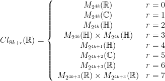
Corollary 7 (Bott Periodicity) As a consequence of (iv) we have $\displaystyle Cl_{n}(\mathbb{C}) = M_{2^{n}}(\mathbb{C})$

if ${n}$ even, and $\displaystyle Cl_{n}(\mathbb{C}) = M_{2^{n}}(\mathbb{C}) \times M_{2^{n}}(\mathbb{C})$

if ${n}$ is odd.

Let’s work out the case when the underlying field is ${\mathbb{R}}$ . For any field ${k}$ we have the following isomorphisms.

Lemma 8 For any field ${k}$

${Cl_{n+2,0}(k) \cong Cl_{0,n}(k) \otimes Cl_{2,0}(k) .}$

${ Cl_{o,n+2}(k) \cong Cl_{n,0}(k) \otimes Cl_{0,2}(k).}$

Proof: Let ${e_{i}}$ denote the standard basis of ${k^{n+2}}$ and cannonical generatoring set of the Clifford algebra ${ Cl_{n+2,0}(k)}$ .

To get the first isomorphism we simply produce a map given by sending $\displaystyle e_{i} \mapsto e_{i} \otimes e_{i}e_{2} \forall 1\leq i \leq n$ and $\displaystyle e_{n+1} \mapsto 1 \otimes e_{1}$ $\displaystyle e_{n+2} \mapsto 1 \otimes e_{2}$ It is easy to check that the above map is an isomorphism.
is similar to ${(i)}$ .

$\Box$ One can explicitly check some of the lower dimension cases( ${ n = 0, 1, 2}$ ). Then one can repeatedly use the isomorphisms in previous lemma. One has to work upto dimension ${8}$ when ${k= \mathbb{R}}$ , before one sees the pattern, which is called the Bott periodicity. Some of the calculations are as follows calculations are as follows

${Cl_{0,0}(\mathbb{R}) \cong \mathbb{R}}$
${Cl_{1,0}(\mathbb{R})\cong \mathbb{C}}$
${Cl_{0,1}(\mathbb{R}) \cong \mathbb{R} \times \mathbb{R}}$
${Cl_{2,0}(\mathbb{R}) \cong \mathbb{H}}$
${Cl_{0,2}(\mathbb{R}) \cong M_{2}(\mathbb{R})}$
${Cl_{3,0}(\mathbb{R}) \cong Cl_{0,1}(\mathbb{R}) \otimes Cl_{2,0}(\mathbb{R})\cong (\mathbb{R} \times \mathbb{R})\otimes \mathbb{H}\cong \mathbb{H}\times \mathbb{H} }$
${Cl_{4,0}(\mathbb{R}) \cong Cl_{0,2}(\mathbb{R}) \otimes Cl_{2,0}(\mathbb{R})\cong M_{2}(\mathbb{R})\otimes \mathbb{H}\cong M_{2}(\mathbb{H}) }$
In general one gets,
${Cl_{n+4,0}(\mathbb{R}) \cong Cl_{0,n+2}(\mathbb{R}) \otimes Cl_{2,0} \cong Cl_{n,0}(\mathbb{R}) \otimes Cl_{0,2}(\mathbb{R}) \otimes Cl_{2,0}(\mathbb{R})}$

Putting all these observations together we get

Theorem 9 The Bott periodicity in case of real number looks like $\displaystyle Cl_{8k+r}(\mathbb{R}) = \left\lbrace \begin{array}{cccccc} M_{2^{4k}}(\mathbb{R})& r=0\\ M_{2^{4k}}(\mathbb{C})& r=1\\ M_{2^{4k}}(\mathbb{H})& r=2\\ M_{2^{4k}}(\mathbb{H}) \times M_{2^{4k}}(\mathbb{H})& r=3\\ M_{2^{4k+1}}(\mathbb{H})& r=4\\ M_{2^{4k+2}}(\mathbb{C})& r=5\\ M_{2^{4k+3}}(\mathbb{R})& r=6\\ M_{2^{4k+3}}(\mathbb{R}) \times M_{2^{4k+3}}(\mathbb{R})& r=7\\ \end{array} \right.$

Lemma 10 As ${k}$ -algebras ${Cl_{n}^{0}(k) \cong Cl_{n-1}(k)}$ Proof:The isomorphism is given explicitly by the map induced by sending

$\displaystyle e_{i} \mapsto e_{i}.e_{n}$

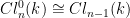
Easy to check that this is an isomorphism of algebras. $\Box$

Written by prasit0605

October 27, 2012 at 6:41 pm

Posted in Uncategorized

Hermitian metrics and Kähler manifolds

leave a comment »

This post will be converted to WordPress soon; in the meantime, view it in PDF form as sections 3 and 4 here: ComplexManifolds

Written by Henry T. Horton

October 25, 2012 at 7:46 pm

Posted in Uncategorized

Complex manifolds and the Dolbeault complex

leave a comment »

This post will be converted to WordPress soon; in the meantime, view it in PDF form as sections 1 and 2 here: ComplexManifolds

Written by Henry T. Horton

October 23, 2012 at 6:28 pm

Posted in Uncategorized

Hodge star operator and Signature operator

leave a comment »

Let $k=\mathbb{R}$ or $\mathbb{C}$ and $V$ be an inner product space with $\{e_1,\cdot\cdot\cdot,e_n\}$ a fixed orthonormal basis, $\Lambda^p V$ be the space of $p$ form

Hodge Star Operator

Lemma 1 There is a unique map $\ast:\Lambda^p V\rightarrow\Lambda^{n-p} V$ s.t. for any $\alpha,\beta\in\Lambda^p V$

$\langle\alpha,\beta\rangle vol=\alpha\wedge\ast\beta$

PROOF. (Uniqueness) suppose we have another map $\ast'$ , then

$\alpha\land(\ast-\ast')\beta=\alpha\land\ast\beta-\alpha\land\ast'\beta=0$ for every $\alpha$

so $(\ast-\ast')\beta=0$ for every $\beta$ ,i.e. $\ast=\ast'$

(Existence) Fix an oriented orthonormal basis $\{e_1,\cdot\cdot\cdot,e_n\}$ , for $\sigma\in S_n$

we define $\ast(e_{\sigma(1)}\land\cdot\cdot\cdot\land e_{\sigma(n)})=\rm{sign}(\sigma)e_{\sigma(p+1)}\land\cdot\cdot\cdot\land e_{\sigma(n)}$

We have $\ast(e_1\land\cdot\cdot\cdot\land e_p)=e_{p+1}\land\cdot\cdot\cdot \land e_{n}$ and $\ast\ast=(-1)^{p(n-1)}$

Suppose $X^n$ is an oriented closed Riemannian Manifold, $\alpha,\beta$ are $p$ forms,define the $l^2$ inner product by

$\langle\alpha,\beta\rangle_{l^2}=\int_{X}\alpha\land\ast\beta$

Using integration by parts and stokes theorem,we have the following equalities:

$\langle d\alpha,\beta\rangle =\int_{X} d\alpha\land\ast\beta$

$= (-1)^p\int_{X} \alpha\land d\ast\beta$

$= (-1)^p\int_{X}\alpha\land (-1)^{(n-p-1)(p+1)}\ast\ast d\ast\beta$

$= \langle\alpha,(-1)^{n(p+1)+1}\ast d\ast\beta\rangle$

hence we yield
Lemma 2 The formal adjoint of $d$ is $\delta=(-1)^{n(p+1)+1}\ast d \ast$ ,i.e. $\langle d\alpha,\beta\rangle=\langle\alpha,\delta\beta\rangle$ .

Exercise Define $\Delta=d\delta+\delta d$ ,show that $\ast\Delta=\Delta\ast$
Corollary $\ast:\mathcal{H}^p\xrightarrow{\cong}\mathcal{H}^{n-p}$

Harmonic Form and Signature

If $\tau:V\rightarrow V$ is an $involution$ and char $F\neq 2$ ,then

$V=V_+\oplus V_{-}$

where $V_{\pm}$ denote the $\pm 1$ eigenspace of $\tau$

If $n=4k$ , $p=2k$ ,then $\ast\ast=1$

Theorem 1 $\mbox{sign}(X)=\dim\mathcal{H}_{+}^p-\dim\mathcal{H}_{-}^p$

PROOF using corollary,we could define the following $nondegenerate$ bilinear form:

$I:\mathcal{H}^p\times\mathcal{H}^p\rightarrow\mathbb{R}\quad(\alpha,\beta)\mapsto\int_{X}\alpha\land\beta$

Let $\mathcal{H}_{\pm 1}^p$ be the $\pm 1$ eigenspace of $\ast$ . For $\alpha\in\mathcal{H}_{+}^p$ , $\beta\in\mathcal{H}_{-}^p$ ,we have:

$I(\alpha,\alpha)=I(\alpha,\ast\alpha)=\langle\alpha,\alpha\rangle\geq0$
$I(\beta,\beta)=-I(\beta,\ast\beta)=-\langle\beta,\beta\rangle\leq 0$
$-I(\alpha,\beta)=\langle\alpha,\beta\rangle=\langle\beta,\alpha\rangle=I(\alpha,\beta)$

Hence there is a decomposation

$\mathcal{H}^p=\mathcal{H}_{+}^p\oplus\mathcal{H}_{-}^p$

and $I$ is positive definite on $\mathcal{H}_+\times\mathcal{H}_+$ and negative definite on $\mathcal{H}_-\times\mathcal{H}_-$

Using Hodge-de Rham isomorphism $\mathcal{H}^p(X)\cong H^p(X,\mathbb{R})$

the above non degenerate bilinear form is equivalent to the intersection form:

$I':H^p(X,\mathbb{R})\times H^p(X,\mathbb{R})\rightarrow\mathbb{R},(\alpha,\beta)\mapsto\langle\alpha\cup\beta,[X]\rangle$

So we have

$\mbox{sign}(X)=\dim H_{+}^p-\dim H_{-}^p=\dim\mathcal{H}_{+}^p-\dim\mathcal{H}_{-}^p$

Signature Operator

If $n=2l$ ,then $\ast\ast=(-1)^{p(n-p)}=(-1)^p$

Let $\Omega^p=C^{\infty}(\Lambda^p T_{\mathbb{C}}^{\ast}X^{2l})$ be the complex-valued $p$ forms,define

$\tau=i^{p(p-1)+n/2}\ast:\Omega^p\rightarrow\Omega^{n-p}$

we have $\tau^2=Id$ and $(d+\delta)\tau=-\tau(d+\delta)$

so if we write $\Omega^{\ast}=\Omega_{+}^{\ast}\oplus\Omega_{-}^{\ast}$ ,where $\Omega_{\pm 1}^{\ast}$ denotes the $\pm 1$ -eigenspace of $\tau$ ,then $D=d+\delta$ interchanges $\Omega_{\pm 1}^{\ast}$ , due to its anti-commutitivity with $\tau$ , i.e.:

$D=d+\delta=\begin{bmatrix} 0 & D_{-} \\ D_{+} & 0 \end{bmatrix}: \Omega_{+}^{\ast}\oplus\Omega_{-}^{\ast}\rightarrow\Omega_{+}^{\ast}\oplus\Omega_{-}^{\ast}$

Definition $D_{+}:\Omega_{+}^{\ast}\rightarrow\Omega_{-}^{\ast}$ is called the signature operator

Theorem 2 $\mbox{Index}(D_{+})=\mbox{sign}(X)$

PROOF we have following facts:

$(d+\delta)^2=\Delta$ is elliptic,hence $d+\delta$ is elliptic,so are $D_{+}$ and $D_{-}$ . $\dim (\mbox{ker} D_{+})$ and $\dim (\mbox{ker} D_{-})$ are finite
$D$ is self-adjoint,so $(D_{+})^{\ast}=D_{-}$
$\mbox{ker} (d+\delta)$ = $\mbox{ker}\Delta$ .so $\mbox{ker} D_{\pm 1}$ consists of harmonic forms for the $\pm 1$ eigenvectors of $\tau$
$\dim\mathcal{H}_{+}^p=\dim\mathcal{H}_{-}^{n-p}$ for $p\neq l$

Using these facts,we yield: $\mbox{Index} (D_{+}) = \dim (\mbox{ker} D_{+})-\dim(\mbox{coker} D_{+})$

$=\dim(\mbox{ker}D_{+})-\dim(\mbox{ker} D_{+}^{\ast})$

$=\dim(\mbox{ker}D_{+})-\dim(\mbox{ker} D_{-})$

$=\Sigma_p\dim\mathcal{H}_{+}^p-\Sigma_p \dim\mathcal{H}_{-}^p$

$=\dim\mathcal{H}_{+}^{l}-dim\mathcal{H}_{-}^{l}$

$=\mbox{sign}(X)$

Written by hailhu

October 21, 2012 at 4:13 pm

Posted in Uncategorized

The Algebraic Hodge Theorem and the Fundamental Theorem of Elliptic Operators

leave a comment »

Statement of the Fundamental Theorem of Elliptic Operators

Definition. Let $V$ and $W$ be inner product spaces. Let $L: V\rightarrow W$ be a linear map. Then a linear map $L^*: W\rightarrow V$ is called the formal adjoint of $L$ if $\langle Lv,w\rangle=\langle v,L^* w\rangle$ for any $v\in V$ and any $w\in W$ .

Lemma. (1) If a formal adjoint exists, it is unique. (2) If $\dim V<\infty$ , then $L^*$ exists.

Example. The map $L: \Bbb{R}^\infty \rightarrow \Bbb{R}$ defined by summing the coodinates has no formal adjoint, where $\Bbb{R}^\infty$ is the colimit of $\Bbb{R}^n$ .

If $V$ and $W$ are Hilbert spaces, then we have

Theorem. Any continuous linear map $L:V\rightarrow W$ of Hilbert spaces has a formal adjoint.

Example. Let $D:C^\infty (E) \rightarrow C^\infty (F)$ be a differential operator. Suppose $E, F$ and $T X$ have smooth inner product structures, then we have the “ $L^2$ -inner products” on $C^\infty (E)$ and $C^\infty (F)$ , given by $\langle s_1,s_2\rangle :=\int_X \langle s_1, \overline{s_2}\rangle$ . Then $D$ has a formal adjoint $D^*:C^\infty (F) \rightarrow C^\infty (E)$ . If we write $D$ locally as $\Sigma A_\alpha (x) D^\alpha$ , then $D^* t=\Sigma (-1)^{|\alpha|} D^\alpha (\overline{A_\alpha}^{tr}t)$ .

An elliptic operator $D: C^\infty(E) \to C^\infty(E)$ is self-adjoint if $D = D^*$ .

We can now state the Fundamental Theorem of Elliptic Operators. Later in this entry we will give some corollaries and much later in the course we will outline a proof using the method of elliptic regularity.

Fundamental Theorem of Elliptic Operators. For a self-adjoint elliptic operator $D : C^\infty(E) \to C^\infty(E)$ , there is an orthogonal decomposition $C^\infty(E) = \ker D \oplus \mathrm{im } D$ with $\ker D$ finite-dimensional.

It is important here that the manifold $X$ is closed.

The algebraic Hodge theorem

Suppose now we have (co)chain complex $(C^\cdot,d)$ over $\Bbb{R}$ or $\Bbb{C}$ :

$\dots \rightarrow C^{p-1} \xrightarrow{d} C^p\xrightarrow{d} C^{p+1}\rightarrow \cdot\cdot\cdot$

Give each $C^p$ an inner product. Assume each $d$ has a formal adjoint $d^*$ . Define the Laplacian $\Delta :=d d^*+d^* d:C^p\rightarrow C^p$ . Then we have

Lemma. $\Delta\alpha=0$ iff $d\alpha=0$ and $d^*\alpha =0$ .

Proof. Suppose $\Delta\alpha =0$ . Then we have

$0=\langle (d d^*+d^* d) \alpha, \alpha\rangle=\langle dd^*\alpha, \alpha\rangle +\langle d^* d\alpha,\alpha\rangle =\langle d^*\alpha, d^*\alpha\rangle +\langle d\alpha,d\alpha\rangle,$

and hence $d\alpha=d^*\alpha=0$ .

$\Box$

Theorem. Let $(C^\cdot,d)$ be a (co)chain complex over a field $k$ . Then there exist decompositions $C^p=H^p\oplus B^p \oplus \hat{B}^p$ such that the (co)chain complex can be written as

$\Box$

When $k=\Bbb{R}$ or $\Bbb{C}$ and $C^p$ is finite dimensional for each $p$ , setting $B^p=\mathrm{Im}\ d$ and $\hat{B}^p=\mathrm{Im}\ d^*$ , the theorem above becomes a corollary of the following Algebraic Hodge Theorem:

Algebraic Hodge Theorem. Let $(C^\cdot,d)$ be a (co)chain complex over $\Bbb{R}$ or $\Bbb{C}$ . Suppose that $C^p$ has inner product for each $p$ and that formal adjoint $d^*:C^{p+1}\rightarrow C^p$ exists for each $p$ . Let $\mathcal{H}^p=\ker\Delta :=dd^*+d^*d:C^p\rightarrow C^p$ , then

(1) TFAE: (a) $\Delta\alpha=0$ , (b) $d\alpha=0$ and $d^*\alpha=0$ , (c) $(d+d^*)\alpha=0$ .

(2) $\Delta(C^p)\subset (\mathcal{H}^p)^\perp$ .

(3) If $C^p$ is finite dimensional, then $C^p=\Delta(C^p)\oplus \mathcal{H}^p$ .

(4) If $C^p=\Delta(C^p)\oplus\mathcal{H}^p$ for any $p$ , then there are orthogonal decompositions

$C^p=\mathcal{H}^p\oplus d(C^{p-1})\oplus d^* (C^{p+1})=\mathcal{H}^p\oplus dd^*(C^p)\oplus d^* d(C^p).$

Proof. (1) (a) $\Rightarrow$ (b) $\Rightarrow$ (c) $\Rightarrow$ (a).

(2) Let $\beta \in \mathcal{H}^p$ , then $\langle \Delta\alpha, \beta\rangle=\langle\alpha,\Delta\beta\rangle=0$ .

(3) Show the inclusion in (2) is an equality by counting dimensions.

(4) It suffices to show the following orthogonal decomposition:

$\Delta (C^p)=d(C^{p-1})\oplus d^*(C^{p+1}) = dd^* (C^p)\oplus d^* d(C^p).$

However easily we have

$\Delta(C^p)\subset dd^*(C^p)\oplus d^*d(C^p)\subset d(C^{p-1})\oplus d^*(C^{p+1})\subset (\mathcal{H}^p)^\perp=\mathrm{Im}\ \Delta.$

$\Box$

By checking the decomposition diagram above, we can obtain:

Corollary. $\phi : \mathcal{H}^p=\ker \Delta \rightarrow H^p(C^\cdot,d)$ is an isomorphism, where $\phi(\alpha)=[\alpha].$

Corollary. $H^*(C^\cdot,d)=0$ iff $\Delta: C^p\rightarrow C^p$ is an isomorphism for any $p$ .

Wrapping up

Corollary. Algebraic Wrapping up. For $(C,d)$ as above: $H^*(C^\cdot,d)=0 \Rightarrow d+d^*: C^{even} =: \oplus C^{2i}\rightarrow C^{odd}=: \oplus C^{2i+1}$ is an isomorphism. Hence $\Delta : C^p \to C^p$ is an isomorphism for all p.

This corollary “wraps up” a (co)chain complex into a single map.

Next, we consider wrapping up an ellliptic complex.

Definition. An elliptic complex of differential operators is a cochain complex of differential operators

$0 \to C^\infty(E^0) \xrightarrow{D} C^\infty(E^1) \xrightarrow{D} \cdots \xrightarrow{D} C^\infty(E^k) \to 0$

so that for all $0\neq\xi\in T_x^*X$ the associated symbol complex is exact.

If we define the symbol of differential operator $D$ of order $m$ by $\sigma_D(x,\xi):=(-i)^m\Sigma_{|\alpha|=m}A_\alpha \xi^\alpha$ , then we have $(\sigma_D)^*=\sigma_{D^*}$ .

Proposition. Let $(C^\infty E^\cdot, D)$ be an elliptic complex of differential operators. Give $E^p$ and $TX$ metrics for each $p$ . Then $D+D^*:C^\infty E^{even}\rightarrow C^\infty E^{odd}$ is an elliptic operator.

Proof. For any $0\neq\xi\in T_x^*X$ , since the complex is elliptic, we have the exact sequence

$\dots\rightarrow E_x^{p-1}\rightarrow E_x^p\xrightarrow{\sigma_p(\xi)} E_x^{p+1}\rightarrow\dots$

Thus, $\sigma_D+(\sigma_D)^*:E_x^{even}\rightarrow E_x^{odd}$ is an isomorphism.

Finally note that $\sigma_D+(\sigma_D)^*=\sigma_D+\sigma_{D^*}=\sigma_{D+D^*}$ .

$\Box$

Consequences of the fundamental theorem.

We deduce the following corollaries of the Fundamental Theorem, the Algebraic Hodge Theorem, and Wrapping Up.

Corollary. Let $(C^\infty(E),D)$ be an elliptic complex of differential operators.

(1) For any $p$ , $\mathcal{H}^p:=\ker \Delta : C^\infty E^p\rightarrow C^\infty E^p$ is finite dimensional.

(2) For any $p$ , $C^\infty E^p=\mathrm{Im}\ \Delta \oplus\mathcal{H}^p$ .

(3) $\mathrm{Index}\ (D+D^*: C^\infty(E^{even}) \to C^\infty(E^{odd}) ) =\Sigma (-1)^p \mathrm{dim}\ \mathcal{H}^p$ .

Corollary. If $D: C^\infty E \rightarrow C^\infty F$ is an elliptic differential operator, then we have isomorphisms $\ker\ D \xrightarrow{\cong} \mathrm{cok}\ D^*, \ker\ D^*\xrightarrow{\cong} \mathrm{cok}\ D$ . Hence the kernel and the cokernel of an elliptic differential operator are finite dimensional.

Corollary. If $D: C^\infty E \rightarrow C^\infty E$ is self-adjoint, then $\mathrm{Index}\ D=0$ .

Written by topoclyb

October 19, 2012 at 6:29 pm

Posted in Uncategorized

Symbols

leave a comment »

This post contains various definitions of the symbol of a differential operator. We will state a local version, then a global version and then we will finally view the symbol in its most abstract form: a section of a bundle over the total space of a cotangent bundle.

Review of Local Definitions

Let’s start by recalling that a differential operator of order ${m}$ on the manifold is ${X={\mathbb R}^n}$ is defined by:

$\displaystyle D=\sum_{|\alpha|\leq m}A_\alpha(\hspace{1ex})D^\alpha:\:C^\infty({\mathbb R}^n,{\mathbb R}^N)\rightarrow C^\infty({\mathbb R}^n,{\mathbb R}^N)\ \ \ \ \ (1)$

where ${A_\alpha(\hspace{1ex}): X={\mathbb R}^n\rightarrow M_{M\times N}({\mathbb R})}$ is smooth and if ${\alpha=(\alpha_1,\ldots,\alpha_n)}$ , then $D^\alpha=\frac{\partial^{\alpha_1}}{\partial x_1^{\alpha_1}}\frac{\partial^{\alpha_2}}{\partial x_2^{\alpha_2}}\cdots\frac{\partial^{\alpha_n}}{\partial x_n^{\alpha_n}}$

Let ${x\in X={\mathbb R}^n}$ and ${\xi\in{\mathbb R}^n=T^*X}$ .  The Symbol of ${D}$ , denoted by ${\sigma_D}$ is then

$\displaystyle \sigma_D(x,\xi)=\sum_{|\alpha|\leq m}A_\alpha(x)\xi_1^{\alpha_1}\xi_2^{\alpha_2}\cdots\xi_n^{\alpha_n}\quad\in M_{M\times N}({\mathbb R})=\text{Hom}({\mathbb R}^N,{\mathbb R}^M)$

A differential operator ${D:\:C^\infty({\mathbb R}^n,{\mathbb R}^N)\rightarrow C^\infty({\mathbb R}^n,{\mathbb R}^N)}$ is said to be elliptic if for all ${x\in X}$ and every ${\xi\neq 0}$ we have that ${\sigma_D(x,\xi)}$ is invertible.

Global definition of the Symbol

Consider a globally defined differential operator

$\displaystyle D:\: C^\infty(E)\rightarrow C^\infty(F)$

for ${x_0\in X}$ and ${\xi\in T_{x_0}^*X}$ we want to define a linear map
$\displaystyle \sigma_D(x_0,\xi):E_{x_0}\rightarrow F_{x_0}$
in a coordinate free way.

With this in mind let ${e\in E_{x_0}}$ and choose:
1. ${f:X\rightarrow{\mathbb R}}$ such that ${\mbox{d} f_{x_0}=\xi}$
2. ${s\in C^\infty(E)}$ such that ${s(x_0)=e}$

Then we define

$\displaystyle \sigma_D(x_o,\xi)(e)=\frac{1}{m!}D(f^ms)(x_0)\ \ \ \ \ (2)$

Notice that even though this is a coordinate free definition of the symbol, it is still unclear how it changes in ${x}$ and ${\xi}$ . We will later see that ${\sigma_D}$ is actually smooth on ${(x,\xi)}$ . Before this, we should prove that this definition is in fact independent on the choice of ${f}$ and ${s}$ .

${\sigma_D}$ does not depend on ${f}$

Claim 1 If ${g: X\rightarrow {\mathbb R}}$ is a smooth function such that ${\mbox{d} g_{x_0}=\xi}$ and ${g(x_0)=0}$ , then
$\displaystyle D((f^m-g^m)s)(x_0)=0$

Proof: For any differential operator ${D}$ , any section ${s}$ and any function ${\varphi:X\rightarrow{\mathbb R}}$ ,

$\displaystyle [D,\varphi](s)=D(\varphi s)-\varphi D(s)$

Setting ${\varphi=f^m-g^m}$ we have

$\displaystyle [D,f^m-g^m](s)(x_0)=D((f^m-g^m)s)(x_0)\ \ \ \ \ (3)$

Induction on the order of ${D}$ and (3) will give us the result:

Let ${D\in \text{DO}_0(E,F)}$ , then by definition

$\displaystyle D((f^m-g^m)s)=(f^m-g^m)D(s)$

and so

$\displaystyle D((f^m-g^m)s)(x_0)=0$

Now assume the claim is true for every differential operator of order less than ${m}$ and suppose ${D\in \text{DO}_m(E,F)}$ . By definition, ${[D,f^m-g^m]\in \text{DO}_{m-1}(E,F)}$
Thus, by induction

$\displaystyle [D,f^m-g^m](s)(x_0)=0$

and notice that (3) gives us

$\displaystyle [D,f^m-g^m](s)(x_0)=D((f^m-g^m)s)(x_0)$

so that

$\displaystyle D((f^m-g^m)s)(x_0)=0$

$\Box$

${\sigma_D}$ does not depend on ${s}$

Claim 2 Let ${s_1,s_2\in C^\infty(E)}$ be such that ${e=s_1(x_0)=s_2(x_0)}$ , then
$\displaystyle D(f^m(s_1-s_2))(x_0)=0$

Proof: It is easier if we use the easy direction of Peetre’s Theorem so that we can use the fact that ${D}$ is local, that is

$\displaystyle \text{supp}(Ds)\subseteq \text{supp}(s)$

equivalently

$\displaystyle X\setminus\text{supp}(s)\subseteq X\setminus\text{supp}(Ds)$

equivalently

$\displaystyle s(x_0)=0\Rightarrow Ds(x_0)=0$

So, since ${f^m(s_1-s_2)(x_0)=0}$ , we have ${D(f^m(s_1-s_2))(x_0)=0}$ as sought. $\Box$

Let us finish the section with a short remark:

${\sigma_D(x_0,\xi)}$ is homogeneous of degree ${m}$ in ${\xi}$ . That is, for every ${\rho>0}$ ,
$\displaystyle \sigma_D(x_0,\rho\xi)=\rho^m\sigma_D(x_0,\xi)$

Proof: Simply take ${\rho f}$ instead of ${f}$ in the definition for ${\sigma_D}$ . $\Box$

Local=Global

Lemma 1 For ${D=\sum_{|\alpha|\leq m}A_\alpha(\hspace{1ex})D^\alpha:\:C^\infty({\mathbb R}^n,{\mathbb R}^N)\rightarrow C^\infty({\mathbb R}^n,{\mathbb R}^N)}$ a differential operator of order ${m}$ , the two definitions of symbol coincide under the identification ${{\mathbb R}^n\cong T_{x_0}^*{\mathbb R}^n}$ given by ${\xi\rightarrow\sum_{i=1}^n\xi_i\mbox{d} x_i}$

Proof: Let ${x_0,\xi\in{\mathbb R}^n}$ . The function ${f(x)=\langle x-x_0,\xi\rangle}$ satisfies the conditions stated in the coordinate free definition of ${\sigma_D}$ .  Let ${s}$ be the constant section ${e}$ , that is, ${s(x)=e}$ for every ${x\in X}$ .

Then (2) reads

$\displaystyle \sigma_D(x_0,\xi)=\frac{1}{m!}D(f^me)(x_0)$

where by (1)

$\displaystyle \frac{1}{m!}D(f^me)(x_0)=\frac{1}{m!}\sum_{|\alpha|\leq m}A_\alpha(x_0)D^\alpha(f^me)(x_0)=\frac{1}{m!}\sum_{|\alpha|\leq m}A_\alpha(x_0)\frac{\partial^{\alpha_1}}{\partial x_1^{\alpha_1}}\frac{\partial^{\alpha_2}}{\partial x_2^{\alpha_2}}\cdots\frac{\partial^{\alpha_n}}{\partial x_n^{\alpha_n}}(f^me)(x_0)$

Notice that here

$\displaystyle D^\alpha(f^me)=\left(\begin{array}{c}D^\alpha(f^me_1)\\D^\alpha(f^me_2)\\ \vdots\\ D^\alpha(f^me_N)\end{array}\right)= \left(\begin{array}{c}D^\alpha(f^m)e_1\\D^\alpha(f^m)e_2\\ \vdots\\ D^\alpha(f^m)e_N\end{array}\right)= D^\alpha(f^m)e$

since ${e}$ is a constant section.

Also notice that
1. ${D^\beta(f^m)(x_0)=0}$ for every ${|\beta|\leq m-1}$ : This is because there is always a factor of ${f}$ in the expression for ${D^\beta(f^m)}$ whenever ${|\beta|\leq m-1}$ .
2. ${D^\alpha(f^m)(x_0)=m!\,\xi_1^{\alpha_1}\xi_2^{\alpha_2}\cdots\xi_n^{\alpha_n}}$ : This is a simple calculation.

Consolidating all the information we conclude

$\displaystyle \sigma_D(x_0,\xi)=\frac{1}{m!}D(f^me)(x_0)=\frac{1}{m!}\sum_{|\alpha|= m}A_\alpha(x_0)D^\alpha(f^me)(x_0)=\sum_{|\alpha|= m}A_\alpha(x_0)\xi_1^{\alpha_1}\xi_2^{\alpha_2}\cdots\xi_n^{\alpha_n}$

$\Box$

Symbol as a section

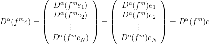
By consolidating definitions (*) and (1) of ${\sigma_D}$ we get ${\sigma_D\in C^{\infty}(\pi^*(\text{Hom}_{\mathbb R}(E,F)))}$ . Here ${\pi}$ is the bundle map ${\pi:T^*X\rightarrow X}$ and we are just looking at the diagram

To be explicit, if ${\omega\in T^*X}$ , then ${\omega=(x_0,\xi)}$ with ${\xi\in T_{x_0}^*X}$ . So

$\displaystyle \sigma_D(\omega)=\sigma_D(x_0,\xi): E_{x_0}\rightarrow F_{x_0}$

that is, ${\sigma_D(x_0,\xi)\in \text{Hom}_{\mathbb R}( E_{x_0}, F_{x_0})}$ and we are using the identification ${\text{Hom}_{\mathbb R}( E_{x_0}, F_{x_0})\cong\pi^*(\text{Hom}_{\mathbb R}( E_{\omega}, F_{\omega}))}$ .

Smoothness follows from the smoothness of the local definition and the fact that both definitions coincide locally.

Finally, let

$\displaystyle \text{sym}_m(E,F)=\{\sigma\in C^{\infty}(\pi^*(\text{Hom}_{\mathbb R}(E,F))) \mid \text{ for all } \rho>0,\: \omega\in T^*X\:,\: \sigma(\rho\omega)=\rho^m\sigma(\omega)\}$

then we have

Proposition 2 There is an exact sequence

$\displaystyle 0\rightarrow \text{DO}_{m-1}(E,F)\rightarrow \text{DO}_{m}(E,F)\rightarrow\text{Symbol}_m(E,F)$

Notice that this proposition (re)captures the fact that the symbol of an operator only `sees’ the `top’ degree of the operator.

Fundamental Theorem of Elliptic Operators

Now that we have a global definition of the symbol of a differential operator, we can state what it means for a differential operator to be elliptic. Namely, ${D}$ is elliptic if for every ${\omega\in T^*X\setminus\{X\}}$ (i.e ${\omega}$ is in the complement of the zero section of the cotangent bundle), the map ${\sigma_D(\omega)}$ is invertible.  The most important result involving elliptic operators is the following theorem:

Theorem 3 Fundamental Theorem of Elliptic Operators
If ${D:\: C^\infty(E)\rightarrow C^\infty(F)}$ is an elliptic differential operator over a compact manifold ${X}$ , then both ${\text{ker}D}$ and ${\text{coker}D}$ are finite dimensional vector spaces.

Written by jpinzon84

September 11, 2012 at 10:42 pm

Posted in Uncategorized

Two beautiful theorems about C(X)

with one comment

Let ${X}$ be a topological space. Let ${C(X)}$ be the ring of continuous functions from ${X}$ to ${\mathbb{R}}$ . ${C(X)}$ can also be thought of as set of smooth sections of the trivial bundle ${ X \times \mathbb{R} \longrightarrow X}$ . Anyway, we get a contravariant functor

$\displaystyle C: Top_* \longrightarrow Ring$

where ${Top}$ is the category of based ${topological}$ ${spaces}$ . ${Ring}$ is the category of ${rings}$ with ${1}$ and every ${ring}$ ${homomorphism}$ sends ${1}$ to ${1}$ . The two beautiful ${theorems}$ to be discussed here are the following.

Theorem 1 (Hewitt) For ${X}$ , ${Y}$ compact Hausdorff there is a bijection

$\displaystyle Top_*(X, Y) \longrightarrow Ring(C(Y), C(X))$

Theorem 2 (Swan) If ${X}$ is compact Hausdorff then taking sections gives a bijection from

$\displaystyle \lbrace \text{ isomorphism class of vector bundles over } X \rbrace \longrightarrow \lbrace \text{finitely generated projective C(X)-modules} \rbrace$

These two beautiful theorems have some remarkable consequences. If ${X}$ , ${Y}$ are compact and Hausdorff then,

$\displaystyle X \cong Y \Longleftrightarrow C(X) \cong C(Y)$

Swan’s Theorem 1 leads to the following result in ${K}$ – ${Theory}$

$\displaystyle K^{0}(X) \cong K_{0}(C(X))$

Theorem 2 is a consequence of the following:

Lemma 1 Let ${X}$ be compact, Hausdorff topological space

For ${x_{0} \in X}$ , $\displaystyle M(x_{0}) = \lbrace f \in C(X): f(x_{0}) = 0 \rbrace$ is a maximal ideal,
If ${M \lhd C(X)}$ is a maximal ideal, then ${\exists !}$ ${x_{0} \in X}$ such that ${M = M(x_{0})}$ ,
${MaxSpec(C(X)) \cong X}$ where ${MaxSpec(R)}$ is the set of all maximal ideals of a ring ${R}$ equipped with ${Zariski}$ topology. The isomorphism takes ${M(x_{0})}$ to ${x_{0}}$

Proof:

Clearly ${M(x_{0})}$ is maximal as ${C(X) / M(x_{0}) \simeq \mathbb{R}}$ which is a field.
Notice, if ${f \notin M(x_{0})}$ , then ${f(x_{0}) \neq 0}$ If ${I}$ is an ${ideal}$ such that ${I \nsubseteq M(x_{0})}$ for all ${x_{0}}$ in ${X}$ then for every ${x \in X}$ , ${\exists}$ ${f_{x} \in I}$ such that ${f_{x}(x) \neq 0}$ . Each ${f_{x}}$ there exists ${U_{x} \ni x}$ such that ${f_{x}(t) \neq 0}$ ${\forall t \in U_{x}}$ . Since ${X}$ is compact ${\lbrace U_{x_{0}}, \ldots U_{x_{n}} \rbrace}$ cover ${X}$ . Using ${bump}$ ${functions}$ ${b_{i}}$ which do not vanish on ${U_{x_{i}}}$ respectively, define $\displaystyle f = |f_{x_{0}}|b_{0} + \ldots +|f_{x_{n}}|b_{n}$ . Observe, ${f(x) \neq 0}$ ${\forall x \in X}$ . Define ${g(x) = \frac{1}{f(x)}}$ . Clearly ${g(x) \in C(X)}$ and ${f.g = 1}$ . Thus ${I = C(X)}$ . Thus the only maximal ideals of ${C(X)}$ is of the form ${M(x_{0})}$ for some ${x_{0} \in X}$ .
For any ideal ${I}$ of a ring ${R}$ define, $\displaystyle V(I) = \lbrace M \text{ maximal in } R : I < M \rbrace$ ${V(I)}$ is the basis for all ${closed}$ sets in the space ${MaxSpec(R)}$ under ${Zariski}$ topology. The map $\displaystyle F : X \longrightarrow MaxSpec(X)$ which sends $\displaystyle x \longmapsto M(x_{0})$
is already a bijection. All we need to show is $\displaystyle C \text{ closed} \Leftrightarrow F(C) \text{ closed}$

${(\Rightarrow):}$
IF ${C}$ closed then define ${I_{C} = \lbrace f \in C(X): f(C) = 0 \rbrace}$ and ${F(C) = V(I_{C}) = \bigcup_{x \in C} M(x)}$ \vspace{5pt}
${(\Leftarrow):}$
IF ${C}$ be a basic closed set in ${MaxSpec(C(X))}$ , ie, ${C= V(I)}$ for some ${I \in C(X)}$ then, define $\displaystyle D = \lbrace x \in X: f(x) = 0 \forall f \in I \rbrace$ . Then ${D}$ is clearly a closed set and clearly ${D = F^{-1}(C)}$ . $\Box$

Proof: (of Theorem 1) In fact the ${C}$ gives the map between the ${Hom}$ sets of the respective category.
One-one
Let ${f: X \longrightarrow Y}$ . Then

$\displaystyle C(f)(g) =f^{*}g = g \circ f$ , where ${g \in C(Y)}$ . If ${C(f) = C(f')}$ then

${\Rightarrow g \circ f = g \circ f' \forall g \in C(Y)}$
${\Rightarrow f(x) = g(x)}$ by using bump functions near each point
Onto
Given a map ${F:C(Y) \longrightarrow C(X)}$ , we induce a map

$\displaystyle \overline{F} : Spec(C(X))\longrightarrow Spec(C(Y))$

By Lemma 1 we get a map

$\displaystyle \overline{F}: X \longrightarrow Y$

It is clear that ${\overline{F}^{*} = F}$ . $\Box$

Proof: ( sketch of proof of theorem 2)
Notice that Let ${G}$ be the map
G: ${\lbrace}$ isomorphism class of vector bundles over ${X}$ ${\rbrace \longrightarrow \lbrace}$ finitely generated C(X)-modules ${\rbrace}$
where given a vector bundle ${\xi}$
${G(\xi)}$ = ${\lbrace}$ smooth sections of ${\xi \rbrace}$ .
Since ${X}$ is compact, any vector bundle ${\xi}$ is a ${subbundle}$ of a trivial bundle of finite dimension, ie ${X \times \mathbb{R}^{n}}$ . Hence ${G(\xi)}$ is a sub-module of ${\bigoplus_{1}^{n} C(X)}$ due to the following isomorphism.
${ \tau: \bigoplus_{1}^{n} C(X) \cong \lbrace }$ smooth sections on the trivial bundle ${X \times \mathbb{R}^{n} \rbrace }$
Thus ${G(\xi)}$ is a finitely generated module. Moreover every bundle ${\xi}$ of finite dimension over a compact space has a complement, say ${\xi^{-1}}$ , hence ${G(\xi) \oplus G(\xi^{-1})=\bigoplus_{1}^{n} C(X)}$ . Hence its projective. Given a finitely generated projective module over ${C(X)}$ , say ${M}$ , find ${n}$ and a ${C(X)}$ module ${N}$ , such that

$\displaystyle M \oplus N = \bigoplus_{1}^{n} C(X)$

Then define ${G^{-1}(M) = \tau^{-1}(M)}$ . This is a ${vector}$ ${bundle}$ over ${X}$ . The proof is non-trivial and is a ${theorem}$ of ${Swan}$ . $\Box$

Written by prasit0605

September 5, 2012 at 1:33 am

Posted in Uncategorized

M721: Index Theory

Examples of Atiyah-Singer Index Theorem

The index theorem for the signature and Dirac operators

The Dirac operator

Clifford algebras and Spin groups

Hermitian metrics and Kähler manifolds

Complex manifolds and the Dolbeault complex

Hodge star operator and Signature operator

The Algebraic Hodge Theorem and the Fundamental Theorem of Elliptic Operators

Symbols

Two beautiful theorems about C(X)

Recent Posts

Archives

Categories

Meta

Share this:

Share this:

Share this:

Share this:

Share this:

Share this:

Share this:

Share this:

Share this:

Share this:

Recent Posts

Archives

Categories

Meta